Text analysis pipeline

Most text mining and NLP modeling use bag of words or bag of n-grams methods. Despite their simplicity, these models usually demonstrate good performance on text categorization and classification tasks. But in contrast to their theoretical simplicity and practical efficiency building bag-of-words models involves technical challenges. This is especially the case in R because of its copy-on-modify semantics.

Let’s briefly review some of the steps in a typical text analysis pipeline:

The researcher usually begins by constructing a document-term matrix (DTM) or term-co-occurrence matrix (TCM) from input documents. In other words, the first step is to vectorize text by creating a map from words or n-grams to a vector space.
The researcher fits a model to that DTM. These models might include text classification, topic modeling, similarity search, etc. Fitting the model will include tuning and validating the model.
Finally the researcher applies the model to new data.

In this vignette we will primarily discuss the first step. Texts themselves can take up a lot of memory, but vectorized texts usually do not, because they are stored as sparse matrices. Because of R’s copy-on-modify semantics, it is not easy to iteratively grow a DTM. Thus constructing a DTM, even for a small collections of documents, can be a serious bottleneck for analysts and researchers. It involves reading the whole collection of text documents into RAM and processing it as single vector, which can easily increase memory use by a factor of 2 to 4. The text2vec package solves this problem by providing a better way of constructing a document-term matrix.

Let’s demonstrate package core functionality by applying it to a real case problem - sentiment analysis.

text2vec package provides the movie_review dataset. It consists of 5000 movie reviews, each of which is marked as positive or negative. We will also use the data.table package for data wrangling.

First of all let’s split out dataset into two parts - train and test. We will show how to perform data manipulations on train set and then apply exactly the same manipulations on the test set:

library(text2vec)
library(data.table)
data("movie_review")
setDT(movie_review)
setkey(movie_review, id)
set.seed(2016L)
all_ids = movie_review$id
train_ids = sample(all_ids, 4000)
test_ids = setdiff(all_ids, train_ids)
train = movie_review[J(train_ids)]
test = movie_review[J(test_ids)]

Vectorization

To represent documents in vector space, we first have to create mappings from terms to term IDS. We call them terms instead of words because they can be arbitrary n-grams not just single words. We represent a set of documents as a sparse matrix, where each row corresponds to a document and each column corresponds to a term. This can be done in 2 ways: using the vocabulary itself or by feature hashing.

Vocabulary-based vectorization

Let’s first create a vocabulary-based DTM. Here we collect unique terms from all documents and mark each of them with a unique ID using the create_vocabulary() function. We use an iterator to create the vocabulary.

# define preprocessing function and tokenization function
prep_fun = tolower
tok_fun = word_tokenizer

it_train = itoken(train$review,
             preprocessor = prep_fun,
             tokenizer = tok_fun,
             ids = train$id,
             progressbar = FALSE)
vocab = create_vocabulary(it_train)

What was done here?

We created an iterator over tokens with the itoken() function. All functions prefixed with create_ work with these iterators. R users might find this idiom unusual, but the iterator abstraction allows us to hide most of details about input and to process data in memory-friendly chunks.
We built the vocabulary with the create_vocabulary() function.

Alternatively, we could create list of tokens and reuse it in further steps. Each element of the list should represent a document, and each element should be a character vector of tokens.

train_tokens = tok_fun(prep_fun(train$review))
it_train = itoken(train_tokens,
                  ids = train$id,
                  # turn off progressbar because it won't look nice in rmd
                  progressbar = FALSE)

vocab = create_vocabulary(it_train)
vocab

## Number of docs: 4000
## 0 stopwords:  ...
## ngram_min = 1; ngram_max = 1
## Vocabulary:
##         term term_count doc_count
##     1:   0.3          1         1
##     2:   0.5          1         1
##     3: 00015          1         1
##     4:   001          1         1
##     5:    03          1         1
##    ---
## 38302:    to      22095      3805
## 38303:    of      23653      3792
## 38304:     a      26614      3878
## 38305:   and      27069      3877
## 38306:   the      54362      3969

Note that text2vec provides a few tokenizer functions (see ?tokenizers). These are just simple wrappers for the base::gsub() function and are not very fast or flexible. If you need something smarter or faster you can use the tokenizers package which will cover most use cases, or write your own tokenizer using the stringi package.

Now that we have a vocabulary, we can construct a document-term matrix.

vectorizer = vocab_vectorizer(vocab)
t1 = Sys.time()
dtm_train = create_dtm(it_train, vectorizer)
print(difftime(Sys.time(), t1, units = 'sec'))

## Time difference of 0.6643901 secs

Now we have a DTM and can check its dimensions.

dim(dtm_train)

## [1]  4000 38306

identical(rownames(dtm_train), train$id)

## [1] TRUE

As you can see, the DTM has rows, equal to the number of documents, and columns, equal to the number of unique terms.

Now we are ready to fit our first model. Here we will use the glmnet package to fit a logistic regression model with an L1 penalty and 4 fold cross-validation.

library(glmnet)
NFOLDS = 4
t1 = Sys.time()
glmnet_classifier = cv.glmnet(x = dtm_train, y = train[['sentiment']],
                              family = 'binomial',
                              # L1 penalty
                              alpha = 1,
                              # interested in the area under ROC curve
                              type.measure = "auc",
                              # 5-fold cross-validation
                              nfolds = NFOLDS,
                              # high value is less accurate, but has faster training
                              thresh = 1e-3,
                              # again lower number of iterations for faster training
                              maxit = 1e3)
print(difftime(Sys.time(), t1, units = 'sec'))

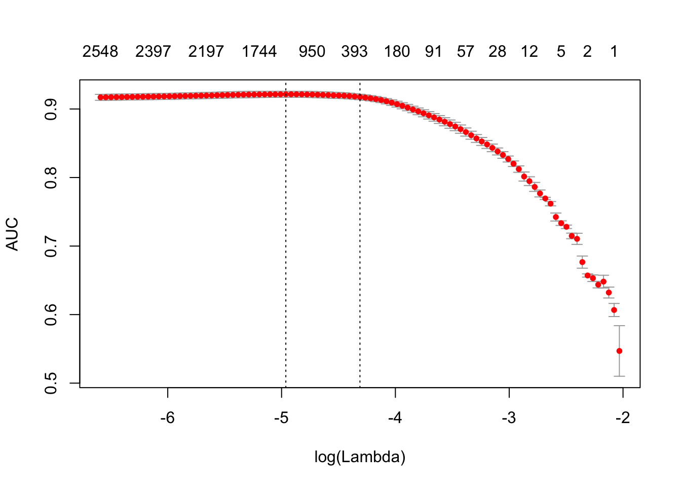
## Time difference of 3.54686 secs

plot(glmnet_classifier)

print(paste("max AUC =", round(max(glmnet_classifier$cvm), 4)))

## [1] "max AUC = 0.9215"

We have successfully fit a model to our DTM. Now we can check the model’s performance on test data. Note that we use exactly the same functions from prepossessing and tokenization. Also we reuse/use the same vectorizer - function which maps terms to indices.

# Note that most text2vec functions are pipe friendly!
it_test = tok_fun(prep_fun(test$review))
it_test = itoken(it_test, ids = test$id,
                 # turn off progressbar because it won't look nice in rmd
                 progressbar = FALSE)

dtm_test = create_dtm(it_test, vectorizer)

preds = predict(glmnet_classifier, dtm_test, type = 'response')[,1]
glmnet:::auc(test$sentiment, preds)

## [1] 0.917393

As we can see, performance on the test data is roughly the same as we expect from cross-validation.

Pruning vocabulary

We can note, however, that the training time for our model was quite high. We can reduce it and also significantly improve accuracy by pruning the vocabulary.

For example, we can find words “a”, “the”, “in”, “I”, “you”, “on”, etc in almost all documents, but they do not provide much useful information. Usually such words are called stop words. On the other hand, the corpus also contains very uncommon terms, which are contained in only a few documents. These terms are also useless, because we don’t have sufficient statistics for them. Here we will remove pre-defined stopwords, very common and very unusual terms.

stop_words = c("i", "me", "my", "myself", "we", "our", "ours", "ourselves", "you", "your", "yours")
t1 = Sys.time()
vocab = create_vocabulary(it_train, stopwords = stop_words)
print(difftime(Sys.time(), t1, units = 'sec'))

## Time difference of 0.3403959 secs

pruned_vocab = prune_vocabulary(vocab,
                                 term_count_min = 10,
                                 doc_proportion_max = 0.5,
                                 doc_proportion_min = 0.001)
vectorizer = vocab_vectorizer(pruned_vocab)
# create dtm_train with new pruned vocabulary vectorizer
t1 = Sys.time()
dtm_train  = create_dtm(it_train, vectorizer)
print(difftime(Sys.time(), t1, units = 'sec'))

## Time difference of 0.3664188 secs

dim(dtm_train)

## [1] 4000 6587

Note that the new DTM has many fewer columns than the original DTM. This usually leads to both accuracy improvement (because we removed “noise”) and reduction of the training time.

Also we need to create DTM for test data with the same vectorizer:

dtm_test   = create_dtm(it_test, vectorizer)
dim(dtm_test)

## [1] 1000 6587

N-grams

Can we improve the model? Definitely - we can use n-grams instead of words. Here we will use up to 2-grams:

t1 = Sys.time()
vocab = create_vocabulary(it_train, ngram = c(1L, 2L))
print(difftime(Sys.time(), t1, units = 'sec'))

## Time difference of 1.533202 secs

vocab = prune_vocabulary(vocab, term_count_min = 10,
                         doc_proportion_max = 0.5)

bigram_vectorizer = vocab_vectorizer(vocab)

dtm_train = create_dtm(it_train, bigram_vectorizer)

t1 = Sys.time()
glmnet_classifier = cv.glmnet(x = dtm_train, y = train[['sentiment']],
                 family = 'binomial',
                 alpha = 1,
                 type.measure = "auc",
                 nfolds = NFOLDS,
                 thresh = 1e-3,
                 maxit = 1e3)
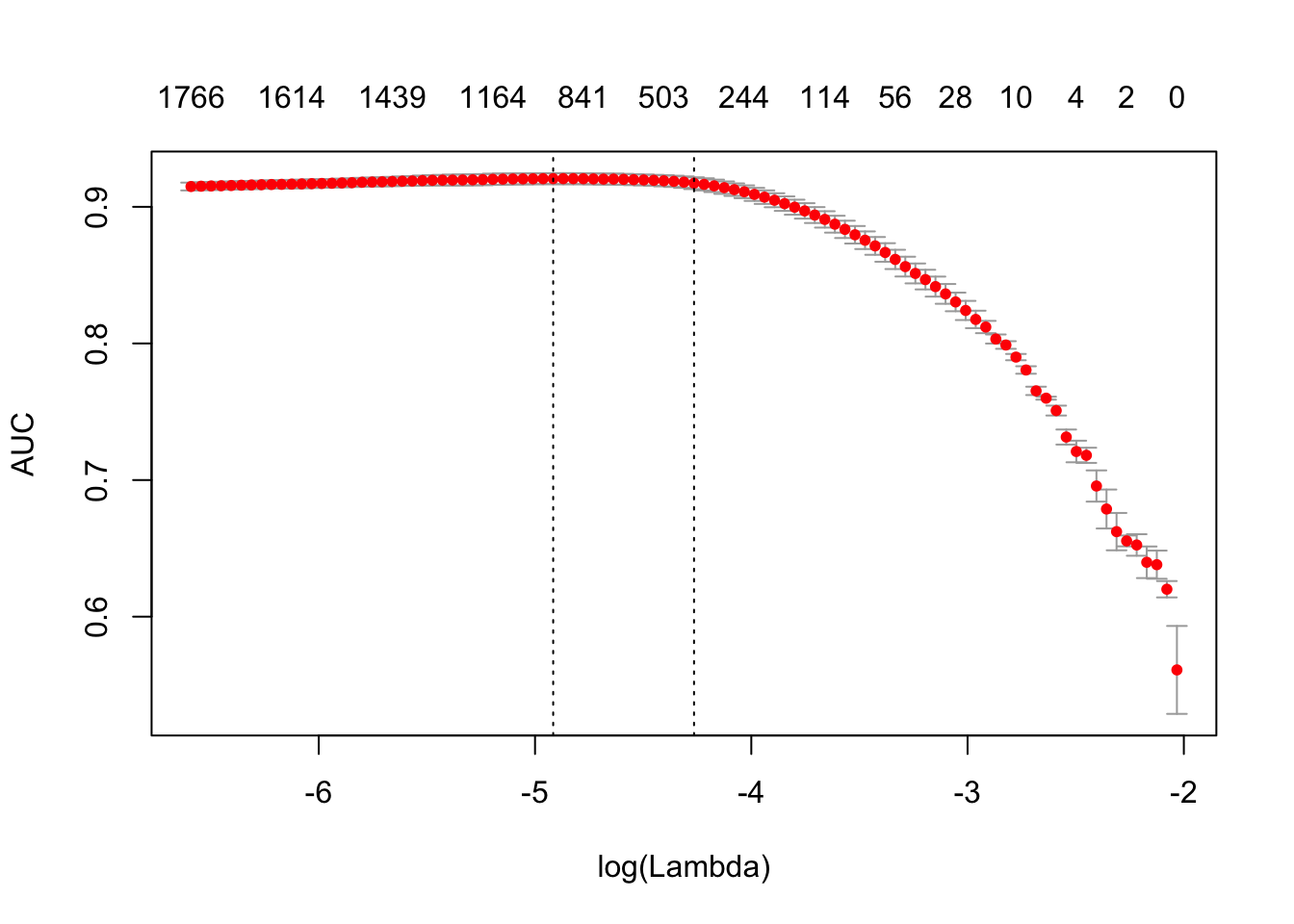
print(difftime(Sys.time(), t1, units = 'sec'))

## Time difference of 2.644238 secs

plot(glmnet_classifier)

print(paste("max AUC =", round(max(glmnet_classifier$cvm), 4)))

## [1] "max AUC = 0.9206"

Seems that usage of n-grams improved our model a little bit more. Let’s check performance on test dataset:

# apply vectorizer
dtm_test = create_dtm(it_test, bigram_vectorizer)
preds = predict(glmnet_classifier, dtm_test, type = 'response')[,1]
glmnet:::auc(test$sentiment, preds)

## [1] 0.9261973

Further tuning is left up to the reader.

Feature hashing

If you are not familiar with feature hashing (the so-called “hashing trick”) I recommend you start with the Wikipedia article, then read the original paper by a Yahoo! research team. This technique is very fast because we don’t have to perform a lookup over an associative array. Another benefit is that it leads to a very low memory footprint, since we can map an arbitrary number of features into much more compact space. This method was popularized by Yahoo! and is widely used in Vowpal Wabbit.

Here is how to use feature hashing in text2vec.

h_vectorizer = hash_vectorizer(hash_size = 2 ^ 14, ngram = c(1L, 2L))

t1 = Sys.time()
dtm_train = create_dtm(it_train, h_vectorizer)
print(difftime(Sys.time(), t1, units = 'sec'))

## Time difference of 0.960351 secs

t1 = Sys.time()
glmnet_classifier = cv.glmnet(x = dtm_train, y = train[['sentiment']],
                             family = 'binomial',
                             alpha = 1,
                             type.measure = "auc",
                             nfolds = 5,
                             thresh = 1e-3,
                             maxit = 1e3)
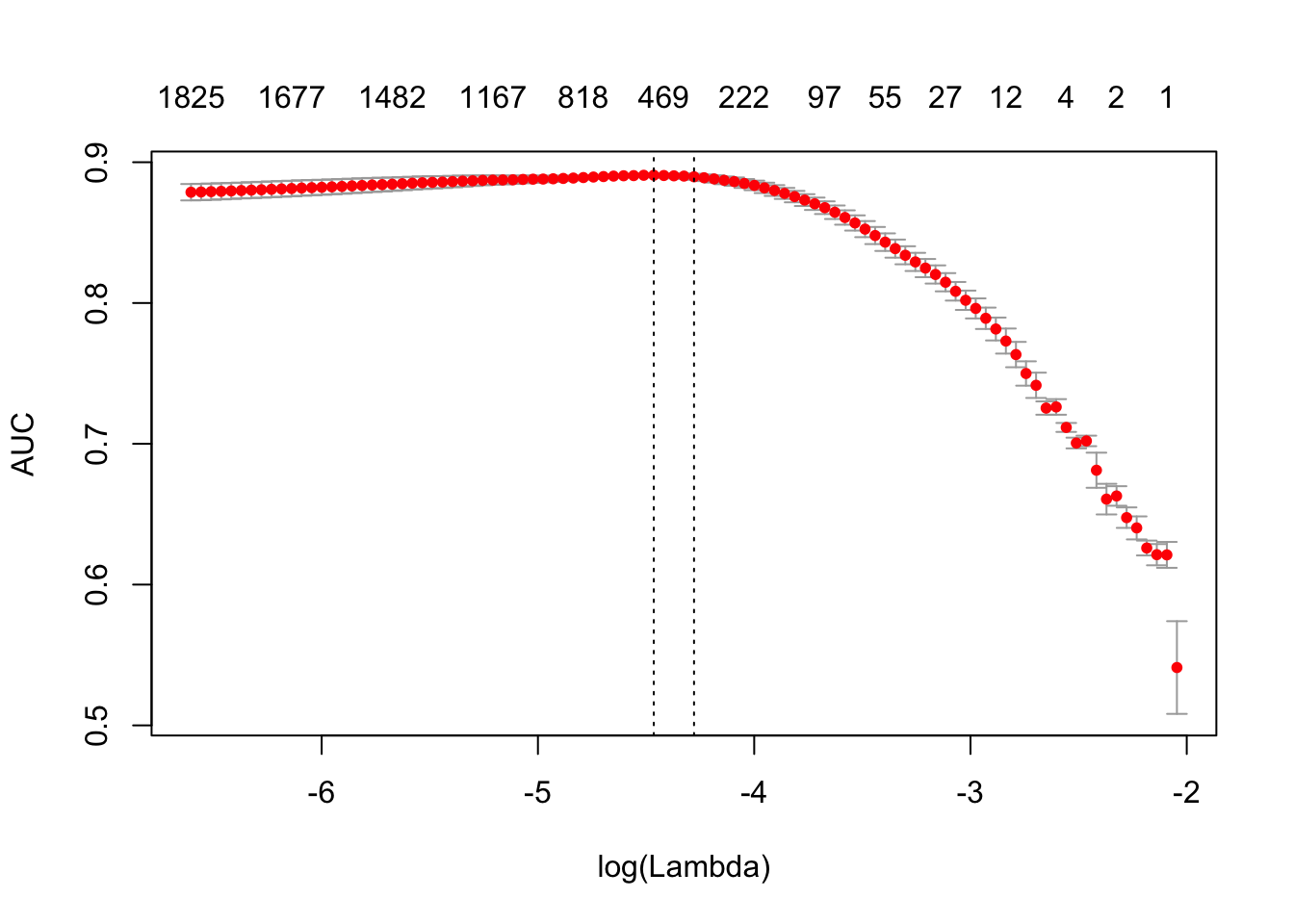
print(difftime(Sys.time(), t1, units = 'sec'))

## Time difference of 4.050237 secs

plot(glmnet_classifier)

print(paste("max AUC =", round(max(glmnet_classifier$cvm), 4)))

## [1] "max AUC = 0.8908"

dtm_test = create_dtm(it_test, h_vectorizer)

preds = predict(glmnet_classifier, dtm_test , type = 'response')[, 1]
glmnet:::auc(test$sentiment, preds)

## [1] 0.9031965

As you can see our AUC is a bit worse but DTM construction time is considerably lower. On large collections of documents this can be a significant advantage.

Basic transformations

Before doing analysis it usually can be useful to transform DTM. For example lengths of the documents in collection can significantly vary. In this case it can be useful to apply normalization.

Normalization

By “normalization” we assume transformation of the rows of DTM so we adjust values measured on different scales to a notionally common scale. For the case when length of the documents vary we can apply “L1” normalization. It means we will transform rows in a way that sum of the row values will be equal to 1:

dtm_train_l1_norm = normalize(dtm_train, "l1")

By this transformation we should improve the quality of data preparation.

TF-IDF

Another popular technique is TF-IDF transformation. We can (and usually should) apply it to our DTM. It will not only normalize DTM, but also increase the weight of terms which are specific to a single document or handful of documents and decrease the weight for terms used in most documents:

vocab = create_vocabulary(it_train)
vectorizer = vocab_vectorizer(vocab)
dtm_train = create_dtm(it_train, vectorizer)

# define tfidf model
tfidf = TfIdf$new()
# fit model to train data and transform train data with fitted model
dtm_train_tfidf = fit_transform(dtm_train, tfidf)
# tfidf modified by fit_transform() call!
# apply pre-trained tf-idf transformation to test data
dtm_test_tfidf = create_dtm(it_test, vectorizer)
dtm_test_tfidf = transform(dtm_test_tfidf, tfidf)

Note that here we first time touched model object in text2vec. At this moment the user should remember several important things about text2vec models:

Models can be fitted on a given data (train) and applied to unseen data (test)
Models are mutable - once you will pass model to fit() or fit_transform() function, model will be modifed by it.
After model is fitted, it can be applied to a new data with fitted_model$transform(new_data) method or equivalent S3 method: transform(new_data, fitted_model).

You can find more detailed overview of models and models API in a separate vignette.

Once we have tf-idf reweighted DTM we can fit our linear classifier again:

t1 = Sys.time()
glmnet_classifier = cv.glmnet(x = dtm_train_tfidf, y = train[['sentiment']],
                              family = 'binomial',
                              alpha = 1,
                              type.measure = "auc",
                              nfolds = NFOLDS,
                              thresh = 1e-3,
                              maxit = 1e3)
print(difftime(Sys.time(), t1, units = 'sec'))

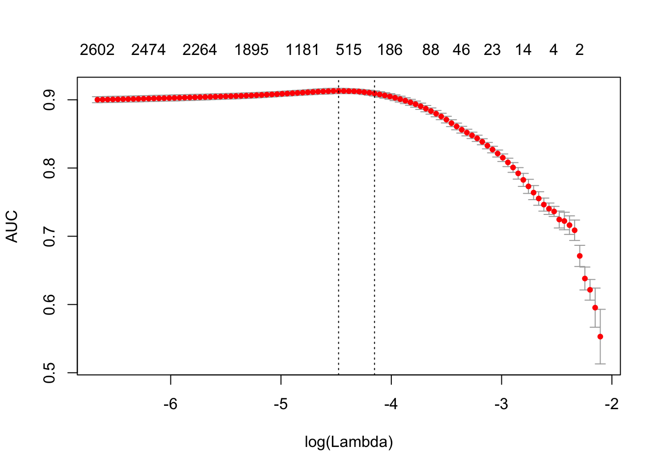
## Time difference of 2.834669 secs

plot(glmnet_classifier)

print(paste("max AUC =", round(max(glmnet_classifier$cvm), 4)))

## [1] "max AUC = 0.913"

Let’s check the model performance on the test dataset:

preds = predict(glmnet_classifier, dtm_test_tfidf, type = 'response')[,1]
glmnet:::auc(test$sentiment, preds)

## [1] 0.9063366

Usually tf-idf transformation significantly improve performance on most of the dowstream tasks.

Vectorization

Dmitriy Selivanov

2018-12-21

Text analysis pipeline

Vectorization

Vocabulary-based vectorization

Pruning vocabulary

N-grams

Feature hashing

Basic transformations

Normalization

TF-IDF